Incorporating NGDP into Taylor rule

Glenn Rudebusch of San Francisco FRB has proposed the following Taylor rule deduced by regression analysis.

FF Rate = 2.07 + 1.28 x Inflation - 1.95 x (Unemployment rate - NAIRU)

Paul Krugman preferred this equation to the original Taylor rule.
The original one can be expressed as follows, according to Taylor's own expression in his Bloomberg column.

FF Rate = 1 + 1.5 x Inflation + 0.5 x GDP gap

There are two merits in Rudebusch version over the original version:

1. Parameters are deduced from actual data, whereas parameters in the original version are rather ad-hoc.


2. Unemployment rate is more straightforward statistics compared to GDP gap.

On this Taylor rule matter, a commenter of this post at "Macro and Other Market Musings" blog made an interesting suggestion.

If you look at the Taylor rule, it does a balancing act between real GDP growth and inflation and only indirectly controls nominal GDP growth. It should be easy to modify the Taylor rule so it would directly control nominal GDP growth by dropping the inflation term and letting the (Yt-Yt*) term represent measured and desired GDPn instead of GDPr. The coefficients would have to be adjusted also.

It would be interesting to compare this modified Taylor rule with the standard Taylor rule over the last few years. Would this modified TR have instructed the Fed to drop the FFR at a faster rate than the standard TR over the past couple of years?

Intrigued by this comment, I defined NGDP-version Taylor rule as follows:

FF Rate = NGDP Growth Rate - 2 x (Unemployment rate - NAIRU)

In this equation, I just replaced constant term and inflation term of Rudebusch version with NGDP Growth Rate, and rounded the coefficient of Unemployment term to nearest integer. It may be crude, but with the merit of simplicity. This equation says that the target rate should be set at minimum rate that suffices dynamic efficiency, once NAIRU is accomplished.

Here is the graph of rate calculated by this version along with Rudebusch version and actual rate:

"FFR" is the actual Federal Fund Rate, "Rule" is the rate calculated by Rudebusch version, "ngdp" is the rate by NGDP version.
As you can see, NGDP version does urge FRB to act more quickly and boldly than either actual FFR or Rudebusch version. And that signal is not limited to past several years. S&L crisis, IT bubble and its burst, housing bubble and its burst,... In every case, NGDP version urged FRB to hike or drop FF Rate more quickly and boldly.


But aren't the parameters of this NGDP-version Taylor rule also ad-hoc? Um, maybe. So, now, let's see what happens if we conduct regression analysis like Rudebusch did, just replacing inflation term in his version with NGDP Growth Rate term. Here is the result:

FF Rate = 3.951 + 0.214 x NGDP Growth Rate - 1.714 x (Unemployment rate - NAIRU)

Unfortunately, adjusted R-squared is not so high... 0.489, as opposed to 0.810 of Rudebusch version. The t-values are not so impressive either... 5.1, 1.6, -6.9, in above order. The t-value of NGDP term is not significant even at 10% level. This result verifies that FRB hasn't considered NGDP Growth Rate as policy target so far. (Maybe it's going to change hereafter, or, so it is hoped.)

Add this NGDP regression version to the above graph, and you get this:


You can see that the movement is rather modified than original NGDP version. However, during 2002-2003 period, this version is the highest among the four.


In fact, if you compare this to what John Taylor asserts FF Rate should have been during this period, it's very close.

The black chain line is what John Taylor asserts as derived from his original version of Taylor rule.

And as for forecast period, i.e. after 2009 Q3, NGDP-Regression version indicates the highest level of FF Rate among three. This also fits what John Taylor asserts in the forementioned Bloomberg column. That is, he asserts that today's ideal FF Rate level is not far from zero, while Krugman and other people says it's lower than -5%. Although NGDP-Regression level is around -4%, it's still nearer to zero than other two rates.


Note: As for data other than NGDP in forecast period, I used Rudebusch's data. NGDP Growth rate in forecast period is set as 2009Q4=0.6%, 2010Q4=3.7%, 2011Q4=4.1% using CBO forecast, and linearly interpolated for intermediate period.


Update(Dec 10, 2009):

　　　　　　　　　　　　　　　　　　　　　　(click to enlarge)

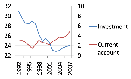
This is what it looks like in Japan. Here, too, NGDP version urges to act more quickly and boldly than either actual policy rate or Rudebusch version.

(I didn't calculate NGDP-Regression version, because that regression is almost meaningless in Japan, which has been caught in liquidity trap for almost 15 years (as you can see in the above graph). I used 3.5% as NAIRU, based on Mr. kuma_asset's estimate. O/N rate became monetary policy tool since 1995 in Japan. Until then, discount rate was the policy rate.)

Paul Krugman's elementary mistakes on economics

In my previous post, I showed that the story of export-led recovery of mid-00's Japan is a myth.

However, there are still many economists who believe that myth. Paul Krugman may be the most famous one among them.

For example, in his April 27 blog post, he showed the following graph.



And he writes,

Here’s Japanese investment and current account balance (trade balance broadly defined), both as a share of GDP, over the period 1992-2007:
Investment was actually lower, as a share of GDP, in 2007 than it had been in 2000. What had changed was the trade balance.

He made two mistakes here.

Mistake No.1

　　What he used as investment is actually Gross Fixed Capital Formation (GFCF).
　　And by definition, it contains Government Investment.

Mistake No.2

　　He failed to recognize that Current account balance and trade balance could be very different.


Let's start with investment. Below is the graph of GFCF and Private Investment (% of GDP).

(source: Cabinet Office HP; click to enlarge)

You can see that while GFCF stagnated after 2003 as Krugman said, Private Investment did increase.

Why this discrepancy occurred? As GFCF consists of Private Investment, Residential Investment, and Public Investment, let's see the movement of each of the component.

Private Investment increased, but the cutback of Public Investment more than offset that increase. The cutback was done because the economy recovered, and budget deficit cannot go on forever. So using GFCF as the sign of lack of investment is total nonsense.


And here is current account and trade balance graph (% of GDP).

(source: Ministry of Finance HP)

Both moved in parallel until 2000, but after that, the movement became very different. Trade balance actually shrank from 2004 till 2006.

The reason of this discrepancy can be also understood by seeing the movement of components.



Income from abroad increased, and that increase was main cause of the discrepancy between current account balance and trade balance.


As a matter of fact, this is not the first time Krugman made mistake on Japanese basic economic statistics. Below is the graph he used in his February 28 post and April 2 post.



And here is the corresponding graph drawn using Japanese SNA statistics. Nominal basis growth is also shown for comparison.


You can see that Krugman is using GFCF as "I" in the above graph, too. And you can see "NX" contribution is next to nothing on nominal basis.

I repeatedly pointed out these facts in his blog comment, but apparently it didn't get through to him.


　

Was recovery of Japanese economy in mid-00's led by export?

No, it wasn't. And here is the reason.


This graph shows that net export did contribute to nominal GDP growth in 2002-2003, but after that, the contribution was marginal. In 2004-2005, the contribution was even negative.

But what is important is real GDP, and net export contributed to that growth, right?

...Um, not necessarily.

Well, it's true that net export contribute to real GDP growth, as I showed in the last graph in my previous post. I'll show the graph again.


This is in stark contrast to the nominal-based graph.

Then, what caused this difference?

Two graphs below answer that question.

(quarterly basis, seasonally adjusted annual rate, billion yen)

On real basis, import did not increase much from 2003 onward, but export did.
On the other hand, both import and export increased on nominal basis, so net export did not change much.

This means that import price hike, caused by the price hike of oil and other natural resources, was what led to contribution of net export to GDP growth on real basis. Of course, it has nothing to do with the increase in export. Yes, export did increase, but that increase was consumed by the increase in import.

In other words, Japan increased export to pay for the hike in price what they import. Otherwise it would have run trade deficit. That situation could be hardly called export-led growth.

Put another way, real GDP growth was somewhat due to net export, but real GDI (Gross Domestic Income) growth wasn't. This is because real GDI is approximately calculated by replacing net export factor from real to nominal. From this point of view, Japan is in contrast to Canada as Prof. Stephen Gordon explained.


　

What happened in Japan in 2003 ?

Below is citation from Krugman's article 10 years ago.

A rigorous model of monetary policy in the face of imperfect substitution is difficult to construct (if only because one must derive that imperfection somehow). But a shortcut may be useful. Consider, then, the case of foreign exchange intervention – purchasing foreign bonds in an effort to bid down the currency. And let us look back at Figure 5, which illustrates how a liquidity trap can occur even in an open economy, because the desired capital export even at a zero interest rate will be less than the excess of domestic savings over investment.

What would the central bank be doing if it engages in exchange-market intervention in such a situation? The answer is that in effect it would be trying to do through its own operations the capital export that the private sector is unwilling to do. So a minimum estimate of the size of intervention needed per year is "enough to close the gap" – that is, the central bank would have to buy enough foreign exchange , i.e. export enough capital, to close the ex ante gap between S-I and NX at a zero interest rate. In practice, the intervention would have to be substantially larger than this, probably several times as large, because the intervention would induce private flows in the opposite direction. (An intervention that weakens the yen reinforces the incentive for private investors to bet on its future appreciation).

Here is some sample arithmetic: suppose that you believe that Japan currently has an output gap of 10 percent, which might be the result of an ex ante savings surplus of 4 or 5 percent of GDP. Then intervention in the foreign exchange market sufficient to close that gap would have to be several times as large as the savings surplus – i.e., it could involve the Bank of Japan acquiring foreign assets at the rate of 10, 15 or more percent of GDP, over an extended period. (Incidentally, does it matter if the interventions are unsterilized? Well, an unsterilized intervention is a sterilized intervention plus quantitative easing; the latter part makes no difference unless it affects expectations).

Thinking about the liquidity trap

Many people think that, in 2003, Japan actually did what Krugman wrote in the above article: i.e. MOF (Ministry of Finance) did huge sum of exchange-market intervention, bid down the currency, and exported enough capital to close the ex ante gap between S-I and NX at a zero interest rate.


Did it really happen? Let's check the data.

Below is the graph of international account. In 2003, huge sum of exchange-market intervention did take place -- although did not exceed 10% of GDP as Krugman suggested, but still reached about 7% of GDP, 34 trillion yen. However, it was only one-year intervention, and was not conducted over an extended period as Krugman suggested.




Did it bid down the currency?
Below is the monthly data of Change in Forex Reserves and JPY/USD exchange rate from 2002 to 2004. You can see that it was far from bidding down the currency -- if anything, all it did was dampen the speed of currency appreciation, at most.




And how did it effect the monetary base?
If you see the below graph carefully, although monetary base increased during 2002-2004, you can see that the increase was not necessarily due to forex intervention. All-out intervention began from mid-2003, but a large part of the increase in monetary base was already made by then.



In sum, the gigantic forex intervention in 2003 did not bid down the currency, and it did not lead to quantitative easing by itself. Then what did it accomplish? Did it close the ex ante gap between S-I and NX?

Maybe. In fact, current surplus increased in 2003. However, the most striking effect of 2003 was that capital account ran large surplus. That is, the intervention caused import of capital, not export of capital as Krugman predicted.

What Krugman suggested as the forex intervention effect was closing the gap between S-I and NX by increasing NX. NX did increase a little, but the most part of the intervetion was consumed by change in capital account, which transformed from deficit to large surplus in 2003. The capital surplus meant that the foreigners invested in Japan, which turned into the increase in I. So if ex ante gap between S-I and NX was closed in Japan, it was caused not by increase in NX as Krugman suggested, but by increase in I!

In other words, the government financed the foreign investment in Japan, which lead to economic recovery. It was not what Krugman predicted. Krugman's theory was that the government finances export, which brings about export-led recovery.

In fact, if you look at the GDP data, you can see that investment was important factor of economic growth on and after 2003. Yes, net export also seems to have played a role, but actually it didn't. I will treat that matter in another post.




　

Weight P/E by P*E ?

A while ago, Jeremy Siegel attacked P/E ratio calculated by S&P for overestimating the real value (here and here. HT Greg mankiw's Blog).

S&P are now using the following formula:


where V_i is the market value and E_i is the earning of issue i, and PER denotes P/E ratio.
Siegel asserts that S&P should weight both market value(numerator) and earning(divisor) by market value, such as:



Siegel says that this weighting will alleviate the problem of overestimating the overall P/E ratio, because the huge loss of the company like AIG will be downplayed by its relatively small market value, in comparison with S&P formula .


However, when you transform S&P formula as follows, you can see that it is also a kind of weighted sum:



That is, individual P/E ratio is weighted by earning.


When you look at Seigel's formula, it can be re-written as follows:



That is, individual P/E ratio is weighted by the product of value and earning.

It can also transformed as follows:


Individual P/E ratio is weighted by the product of P/E and squared earning.

From these transformations, you can see that the meaning of Siegel's formula is much harder to grasp than S&P one.


For Siegel's purpose, maybe it's better to weight individual earning by market value, instead of by earning in S&P formula, as follows:




　

The Geithner put : simulation

In the previous post, I showed the way to simulate Geithner plan by Excel for three probability density functions(uniform, normal, log-normal). In this post, I show some graphs from the simulation.

Here I use log-normal PDF, for it is the most probable function of the three.
Specifically, I assumed that ln(P) follows N[m,s] distribution, and set mean m as ln(100)-s²/2. That means expected value of P (=E[P]) is always set as 100.

• standard deviation simulation

First, change standard deviation s from 0.1 to 1.1 by 0.05. Self financing ratio k is set as 1/7 as in the Geithner plan.

X-axis is the simulation factor s, as described above.
P₁ is the expected price conditional that non-recourse loan not be used.
P₂ is the expected price conditional that non-recourse loan be used.
P_b is the break-even bid price.
p₁(right-hand scale) is the probabaility that non-recourse loan not be used.

As s increases, P₁ and P_b goes up, and P₂ decreases gradually.
p₁ decrease from over 0.9 to near 0.1 for the simulated range of s.


The graph below shows taxpayer's loss (FDIC's loss, to be exact) as percentage of (1-k)P_b(=the value of FIDC non-recourse loan), instead of p₁ for the same simulation (right-hand scale). X-axis is same as above, but numbers are changed from s to s/m (coefficient of variance) so that the meaning of x-axis becomes more easy to grasp.

For coefficient of variance of 0.27, FDIC's loss ratio reaches near 60%.

• non-recourse loan ratio simulation

Next, change self financing ratio k(=1 - non-recourse loan ratio) from 0.05 to 0.95 by 0.05 (this includes Treasury funding). s(standard deviation) is set as 0.5.

(Again, p₁ is right-hand scale.)

When k increases from 0.15 to 0.45, P_b premium to E[P] decreases from 22.0% to 2.3%. Maybe low k value(1/7=14.3%) in the Geithner plan was set in order to provide enough (over 20%) subsidy to the bank.


FDIC's loss ratio is as follows.

(Again, loss ratio is right-hand scale.)

If non-recourse loan ratio (1-k) is about 75% instead of 85.7% in the Geithner plan, the loss drops in half (around 20% to 10%). If (1-k) is 50%, loss becomes less than 3%.


　

The Geithner put : general PDF case

In the previous two posts, I showed general formula of break-even purchase price and fund's gain/loss under the Geithner plan. I also did some arithmetic using two-state model.

Krugman wrote "the natural way to think about these things is in fact in terms of simple two-state numerical examples." Nemo commented "binomial distribution is oversimplified."

However, two-state model may be not so simple as it seems. It can be described as reduced form of more general case.

Let p(P) the probability density function(PDF) of P. Then P₁, P₂, p₁ in the two-state model I used can be derived from p(P) as follows:



where P_b is break-even purchase price, and (1-k) is ratio of non-recourse loan offered by FDIC.

As derived here, P_b is function of P₁ and p₁. That is, P_b = p₁P₁ / (p₁+k(1-p₁)). So P_b and P₁, p₁ must be calculated simultaneously.

As for general PDF, that calculation can be done by Excel. Below I show how to do the calculation by Excel for three forms of p(P), i.e. uniform distribution, normal distribution, log-normal distribution.

• uniform distribution

	p1	P1	Pb
Excel row/column	A	B	C
2	Initial value	Initial value	=A2*B2/(A2+$G$2*(1-A2))
3	=($I$2-C2*(1-$G$2))/($I$2-$H$2)	=($I$2^2-(C2*(1-$G$2))^2)/2/($I$2-$H$2)/A3	=A3*B3/(A3+$G$2*(1-A3))

Input k in G2 cell, and upper limit of uniform distribution in I2 cell, lower limit in H2 cell.
If you drag fill handle of 3rd row to appropriate row (say, 41st row), then each value of P_b, P₁, p₁ will converge.

• normal distribution

	p1	P1	Pb
Excel row/column	A	B	C
2	Initial value	Initial value	=A2*B2/(A2+$G$2*(1-A2))
3	=1-NORMDIST(C2*(1-$G$2),$H$2,$I$2,TRUE)	=(EXP(-((((1-$G$2)*C2-$H$2)/$I$2))^2/2)*$I$2/SQRT(2*PI())+$H$2*A3)/A3	=A3*B3/(A3+$G$2*(1-A3))

Input k in G2 cell, and mean of normal distribution in H2 cell, standard deviation in I2 cell.
If you drag fill handle of 3rd row to appropriate row (say, 41st row), then each value of P_b, P₁, p₁ will converge (if they ever do).

(Note: Above Excel formula is based on normal distribution without restriction, so price could be negative.)

• log-normal distribution

	p1	P1	Pb
Excel row/column	A	B	C
2	Initial value	Initial value	=A2*B2/(A2+$G$2*(1-A2))
3	=1-LOGNORMDIST(C2*(1-$G$2),$H$2,$I$2)	=(1-NORMDIST( (LN(C2*(1-$G$2))-$H$2)/$I$2,$I$2,1,TRUE))*EXP($I$2^2/2+$H$2)/A3	=A3*B3/(A3+$G$2*(1-A3))

Input k in G2 cell, and mean of log-normal distribution in H2 cell, standard deviation in I2 cell.
If you drag fill handle of 3rd row to appropriate row (say, 41st row), then each value of P_b, P₁, p₁ will converge (if they ever do).



　

The Geithner put : option formula

In the previous post , I showed the general formula of break-even purchase price under Geithner plan.

In that post, I showed the gain/loss of the investment fund as follows:
　　　w(P - P_b)　　　if P >= (1-k)P_b
　　　-wP_b　　　　　 if P < (1-k)P_b
where:
P is true price of the loan,
P_b is the purchase price,
(1-k) is ratio of non-recourse loan offered by FDIC (6/7 in case of Geithner plan),
w is ratio of fund money in investment (1/2 in case of Geithner plan; the rest(=1-w) is funded by Treasury).

It also can expressed in option formula as follows:
　　　w{Max(P-P_b , -kP_b)}
　　=w{Max(P-(1-k)P_b , 0)-kP_b}

This is the formula of call option with strike price=-(1-k)P_b and option purchase price=kP_b (See image below).


By applying the above option formula, it can be calculates as
　　　0.5*{(0.5*(100-84*6/7)+0.5*0)-84/7}=1
which corresponds to Nemos's result.

As Nemo showed, the money fund put in is wkP_b=0.5*1/7*84=6. So the fund performance reaches 1/6*100=16.67%.

FDIC gain/loss also can be expressed in option formula as follows:
　　　-Max(0 , (1-k)P_b-P)
(In fact, maximum gain is not zero, as there is interest revenue. Here I ignore it for simplicity)

This is the formula of put option with strike price=-(1-k)P_b (See image below).


The FDIC position is short on this put option, and that "Geithner put" is what enables the floor part of the fund's call option shown above.


　

The Geithner put : general formula

Many people have been calculating the effect of Geithner put in the Geithner plan (aka PPIP) . However, while many have shown numerical examples, seldom of them have shown the general formula. So I am going to give one.

Usually, when a fund purchases loan from bank, its gain/loss can be written as
　　　P - P_b
where P is true price of the loan, and P_b is the purchase price.
Therefore, expected return of the fund becomes zero when P_b=E[P]
(E[.] denotes expectation value).

But with Geithner put, the gain/loss of the fund becomes
　　　w(P - P_b)　　　if P >= (1-k)P_b
　　　-wP_b　　　　　 if P < (1-k)P_b
where:
(1-k) is ratio of non-recourse loan offered by FDIC (6/7 in case of Geithner plan),
w is ratio of fund money in investment (1/2 in case of Geithner plan; the rest(=1-w) is funded by Treasury).

In this case, P_b, the break-even purchase price, is not necessarily E[P].

Now let P becomes P₁ with probability p₁, and P₂ with probability 1-p₁.
(Assumption: P₁ >= (1-k)P_b > P₂)

Then the break-even purchase price can be written as
　　　P_b = p₁P₁ / (p₁+k(1-p₁))

RHS does not include P₂, which means one does not have to consider P₂ as for down-side risk. This is because if down-side event really happens, the price P₂ does not affect the loss of the fund; the fund just loses the money it put in.

Let confirm this formula by Krugman's example. In Krugman's case, p₁=0.5, P₁=150, k=0.15, so P_b becomes 130.43, which corresponds to Krugman's calculation.

Jeffrey Sachs also showed numerical example. His setting is p₁=0.2, P₁=1,000,000, k=0.1. Then P_b becomes 714,268, which corresponds to Sachs's calculation.

And in this case, break-even price P_b is always higher than expectation value of P. That result can be shown by the following arithmetic:

　P_b-E[P]
=p₁P₁ / (p₁+k(1-p₁)) - (p₁P₁+(1-p₁)P₂)
=p₁P₁ [1/{p₁+k(1-p₁)} -1] - (1-p₁)P₂
=p₁P₁[(1-k)(1-p₁)/{p₁+k(1-p₁)}] - (1-p₁)P₂
=(1-p₁)[p₁P₁(1-k)/{p₁+k(1-p₁)} - P₂]
=(1-p₁)[(1-k)P_b-P₂]

This value is always positive by assumption. And this value represents the "subsidy" to the bank under the Geithner plan.

And if the purchase price is higher than break-even price P_b by, say, R, it adds to that subsidy to the bank.
In that case, the private invester loss is -wR(p₁+(1-p₁)k), Treasury loss is -(1-w)R(p₁+(1-p₁)k).
And FDIC loss becomes larger by -R(1-(p₁+(1-p₁)k)).
Graph below shows the loss of the three stake holders as function of p₁ (total=100%; k=1/7, a=1/2 as in the Geithner plan).
　

Loss of FDIC+Treasury makes up 80% of total when p₁=0.3, and becomes less than 70% only when p₁ is larger than 0.6.