The Geithner put : simulation

In the previous post, I showed the way to simulate Geithner plan by Excel for three probability density functions(uniform, normal, log-normal). In this post, I show some graphs from the simulation.

Here I use log-normal PDF, for it is the most probable function of the three.
Specifically, I assumed that ln(P) follows N[m,s] distribution, and set mean m as ln(100)-s²/2. That means expected value of P (=E[P]) is always set as 100.

• standard deviation simulation

First, change standard deviation s from 0.1 to 1.1 by 0.05. Self financing ratio k is set as 1/7 as in the Geithner plan.

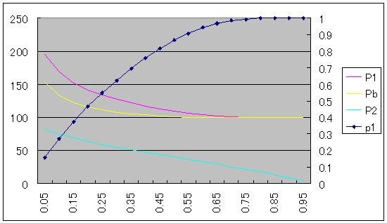
X-axis is the simulation factor s, as described above.
P₁ is the expected price conditional that non-recourse loan not be used.
P₂ is the expected price conditional that non-recourse loan be used.
P_b is the break-even bid price.
p₁(right-hand scale) is the probabaility that non-recourse loan not be used.

As s increases, P₁ and P_b goes up, and P₂ decreases gradually.
p₁ decrease from over 0.9 to near 0.1 for the simulated range of s.


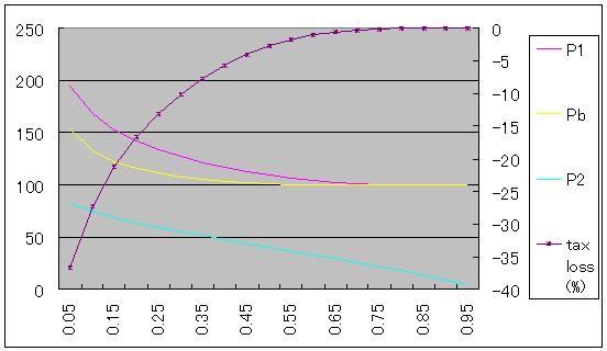
The graph below shows taxpayer's loss (FDIC's loss, to be exact) as percentage of (1-k)P_b(=the value of FIDC non-recourse loan), instead of p₁ for the same simulation (right-hand scale). X-axis is same as above, but numbers are changed from s to s/m (coefficient of variance) so that the meaning of x-axis becomes more easy to grasp.

For coefficient of variance of 0.27, FDIC's loss ratio reaches near 60%.

• non-recourse loan ratio simulation

Next, change self financing ratio k(=1 - non-recourse loan ratio) from 0.05 to 0.95 by 0.05 (this includes Treasury funding). s(standard deviation) is set as 0.5.

(Again, p₁ is right-hand scale.)

When k increases from 0.15 to 0.45, P_b premium to E[P] decreases from 22.0% to 2.3%. Maybe low k value(1/7=14.3%) in the Geithner plan was set in order to provide enough (over 20%) subsidy to the bank.


FDIC's loss ratio is as follows.

(Again, loss ratio is right-hand scale.)

If non-recourse loan ratio (1-k) is about 75% instead of 85.7% in the Geithner plan, the loss drops in half (around 20% to 10%). If (1-k) is 50%, loss becomes less than 3%.